%matplotlib inline
import pandas as pd
import numpy as np
import matplotlib.pyplot as plt
import math

from keras.utils.np_utils import to_categorical
from keras.models import Sequential, load_model, Model
from keras.layers import Dense, Dropout, Flatten, Conv2D, MaxPool2D
MNIST 예제를 수행하기 전에, 필요한 라이브러리들을 임포트합니다.
from keras.datasets import mnist

(x_train, y_train), (x_test, y_test ) = mnist.load_data()
해당 mnist 데이터셋을 다음과 같이 불러옵니다.
plt.imshow(x_train[0], cmap='binary')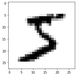
위와 같이 데이터가 잘 나오는지 확인해볼 수 있습니다.
x_train = x_train.reshape(60000, 28, 28, 1)
x_test = x_test.reshape(-1, 28, 28, 1)

y_train = to_categorical(y_train)
y_test = to_categorical(y_test)

x_train = x_train/255.0
x_test = x_test/255.0
이제 다음과 같이 트레인 데이터로 훈련할 수 있도록 형태를 변형합니다. 변형하는 방식은 위와 같습니다.
model = Sequential()
model.add(Conv2D(filters=16, kernel_size=(5,5), padding='valid', strides=1, activation='relu', input_shape=(28,28,1,)))
model.add(MaxPool2D(pool_size=(2,2)))
model.add(Conv2D(filters=36, kernel_size=(5,5), padding='valid', strides=1, activation='relu'))
model.add(Flatten())
model.add(Dense(128, activation='relu'))
model.add(Dense(10, activation='softmax'))
model.summary()

model.compile(loss='categorical_crossentropy', optimizer='adam', metrics=['accuracy'])

"""
WARNING:tensorflow:From C:\Users\user\AppData\Local\Continuum\anaconda3\lib\site-packages\tensorflow\python\framework\op_def_library.py:263: colocate_with (from tensorflow.python.framework.ops) is deprecated and will be removed in a future version.
Instructions for updating:
Colocations handled automatically by placer.
_________________________________________________________________
Layer (type)                 Output Shape              Param #
=================================================================
conv2d_1 (Conv2D)            (None, 24, 24, 16)        416
_________________________________________________________________
max_pooling2d_1 (MaxPooling2 (None, 12, 12, 16)        0
_________________________________________________________________
conv2d_2 (Conv2D)            (None, 8, 8, 36)          14436
_________________________________________________________________
flatten_1 (Flatten)          (None, 2304)              0
_________________________________________________________________
dense_1 (Dense)              (None, 128)               295040
_________________________________________________________________
dense_2 (Dense)              (None, 10)                1290
=================================================================
Total params: 311,182
Trainable params: 311,182
Non-trainable params: 0
"""
이제 모델을 선언해 레이어를 구성합니다. 제가 구성한 레이어는 다음과 같습니다.
model.fit(x_train, y_train, batch_size=200, epochs=10, validation_split=0.2)

"""
WARNING:tensorflow:From C:\Users\user\AppData\Local\Continuum\anaconda3\lib\site-packages\tensorflow\python\ops\math_ops.py:3066: to_int32 (from tensorflow.python.ops.math_ops) is deprecated and will be removed in a future version.
Instructions for updating:
Use tf.cast instead.
Train on 48000 samples, validate on 12000 samples
Epoch 1/10
48000/48000 [==============================] - 6s 121us/step - loss: 0.2607 - acc: 0.9246 - val_loss: 0.0808 - val_acc: 0.9759
Epoch 2/10
48000/48000 [==============================] - 2s 43us/step - loss: 0.0671 - acc: 0.9795 - val_loss: 0.0582 - val_acc: 0.9840
Epoch 3/10
48000/48000 [==============================] - 2s 43us/step - loss: 0.0457 - acc: 0.9860 - val_loss: 0.0552 - val_acc: 0.9848
Epoch 4/10
48000/48000 [==============================] - 2s 50us/step - loss: 0.0345 - acc: 0.9891 - val_loss: 0.0454 - val_acc: 0.9869
Epoch 5/10
48000/48000 [==============================] - 2s 44us/step - loss: 0.0290 - acc: 0.9904 - val_loss: 0.0402 - val_acc: 0.9888
Epoch 6/10
48000/48000 [==============================] - 2s 44us/step - loss: 0.0227 - acc: 0.9930 - val_loss: 0.0420 - val_acc: 0.9882
Epoch 7/10
48000/48000 [==============================] - 2s 47us/step - loss: 0.0166 - acc: 0.9946 - val_loss: 0.0353 - val_acc: 0.9897
Epoch 8/10
48000/48000 [==============================] - 2s 44us/step - loss: 0.0142 - acc: 0.9954 - val_loss: 0.0386 - val_acc: 0.9901
Epoch 9/10
48000/48000 [==============================] - 2s 45us/step - loss: 0.0124 - acc: 0.9960 - val_loss: 0.0437 - val_acc: 0.9886
Epoch 10/10
48000/48000 [==============================] - 2s 47us/step - loss: 0.0104 - acc: 0.9965 - val_loss: 0.0402 - val_acc: 0.9888
"""
이제 해당 훈련 데이터를 넣어주고, 훈련을 진행합니다. 정확도가 거의 99프로 가까이 도달하는 것을 확인할 수 있습니다.
score = model.evaluate(x_test, y_test)
print(score)

"""
10000/10000 [==============================] - 1s 65us/step
[0.036310680392265204, 0.9896]
"""
실제 테스트 데이터를 가지고 백테스팅을 진행해보겠습니다. 만개의 데이터는 9896개를 정확히 예측한 것을 알 수 있습니다.
l1 = model.get_layer('conv2d_1')
l1.get_weights()[0].shape

"""
(5, 5, 1, 16)
"""
이제 구성한 model 레이어에 대해 알아보도록 하겠습니다. 해당 모델의 정보를 가져와 가중치를 가져오는 법은 다음과 같습니다.
def plot_weight(w):
    w_min = np.min(w)
    w_max = np.max(w)

    num_grid = math.ceil(math.sqrt(w.shape[3]))
    fix, axis = plt.subplots(num_grid, num_grid)
    for i, ax in enumerate(axis.flat):
        if 9 < w.shape[3]:
            img = w[:,:,0,i]
            ax.imshow(img, vmin=w_min, vmax=w_max)
        ax.set_xticks([])
        ax.set_yticks([])
    plt.show()
이제 가져온 가중치의 정보를 가시화해보도록 하겠습니다. 함수는 다음과 같습니다.
l1 = model.get_layer('conv2d_1')
w1 = l1.get_weights()[0]
plot_weight(w1)

l2 = model.get_layer('conv2d_2')
w2 = l2.get_weights()[0]
plot_weight(w2)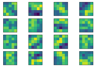
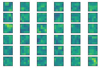
레이어들과 해당 가중치를 다음과 같이 가시화한 결과는 위와 같습니다. 이렇게 잘게 나누어 값들을 판별해서, 이미지 인식을 하는 것을 알 수 있습니다.
temp_model = Model(inputs=model.get_layer('conv2d_1').input, output=model.get_layer('conv2d_1').output)
output = temp_model.predict(x_test)
이제 아웃풋에 대한 결과를 가시화해보도록 하겠습니다. 해당 model의 인풋과 아웃풋을 넣어줍니다. 그 다음, test 데이터를 넣어주었습니다.
def plot_output(output):
    num_grid = math.ceil(math.sqrt(output.shape[3]))

    fix, axis = plt.subplots(num_grid, num_grid)

    for i, ax in enumerate(axis.flat):
        if i < output.shape[3]:
            img = output[0, :, :, i]
            ax.imshow(img, cmap='binary')

        ax.set_xticks([])
        ax.set_yticks([])

    plt.show()
이제 해당 아웃풋을 가시화해줄 함수를 구현해보았습니다.
plot_output(output)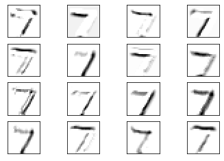
다음과 같이 인풋값을 넣어주고 나온 아웃풋은 가시화하면 다음과 같이 나오는 것을 확인할 수 있습니다. 이것은 즉, 하나의 인풋을 여러개로 나누어, 해당 인풋값의 특징들을 찾아내고, 그 특징들의 값을 토대로 예측하는 CNN 구조를 이해하는 데, 큰 도움이 됩니다.
'SW > 영상인식' 카테고리의 다른 글
| 영상인식 : 케라스 : CIFAR10 : TRANSFER LEARNING : 예제 (6) | 2019.11.07 |
|---|---|
| CIFAR10 : 새로운 클래스 인식, 테스트 데이터 구성 : 실습 (5) | 2019.11.04 |
| CIFAR10 : 정확도 90% : visualization, plotting, 실제 이미지 테스트 (0) | 2019.11.03 |
| CIFAR 10 : Few Shot Learning : 새로운 클래스 인식 (1) | 2019.11.02 |
| 내 손글씨를 직접 mnist 모델에 적용하는 방법 (1) | 2019.10.07 |